Tracking Pavement Smoothness After Each Activity
Jas. W. Glover, Ltd., a materials producer and laydown contractor, in Hawaii collected inertial profiler data on each phase of a project on the Island of Hawaii and implemented different processing techniques to improve final smoothness
Jayanth Kumar Rayapeddi Kumar, P.E.
Quality Control Engineer
Jas. W. Glover, Ltd.
Nick Schaefer, P.E.
Profiling Systems Engineer
Surface Systems and Instruments, Inc.
Introduction
Whether we’re going to work or to a restaurant or traveling for any other reason, we depend on roads every day. We simply can’t do without them. Can we? According to Bureau of Transportation Statistics, the US had about 8.7 million lane-miles of roads and over 2.9 trillion vehicle miles traveled. It is necessary to keep these roads smooth and well-maintained, as they offer a safer and more comfortable driving experience for motorists, reduce vehicle wear, cut down fuel consumption, and contribute to the overall efficiency of the transportation network.
Smoothness can be measured using several different methods. Qualitatively, this can be the comfort of a new pavement where you can drink your coffee without spilling or your vehicle interior doesn’t squeak. Quantitatively, common data collection methods have evolved over time and technology. Almost every pavement project will still require straightedge testing that indicates localized evenness of the pavement surface. A small, decreasing number of agencies still use California Profilograph which measures the Profile Ride Index (PRI). But progressively, more agencies prefer measuring surface smoothness using a vehicle-mounted high-speed inertial profiling system because it’s advantageous to collect data at highway speeds without traffic closures and improved data accuracy and reliability.
Although most highway agencies have transitioned to International Roughness Index (IRI) and inertial profilers, a straightedge specification will always be relevant. Straightedges will always have a place testing locations where an inertial profiler cannot collect data or for inspectors and superintendents to rapidly check joints and transitions before the closure is opened. It is best practice to have a straightedge on hand during milling or paving to visually verify.
Inertial Profilers
Accelerometers and lasers are the primary sensors within inertial profiler systems. The accelerometer cancels out the vertical vehicle suspension movement while the laser measures the vertical displacement from the vehicle to the ground. After combining these two sensors a relative elevation profile is created. To be compliant with ASTM E950 Class I profiler requirements, the longitudinal profile is typically captured at 1-inch intervals.
Additional data streams or upgrades are available on inertial profilers. Options for profiling systems can range from:
- Higher accuracy GPS receivers with corrections to achieve 10mm horizontal accuracy
- INS systems to report cross-slope and running grade
- Right-of-Way cameras to record images
- GPS-DMI’s for distance measurement without calibration
- GPS Navigation to corrective grinding
- Zero-Speed “stop-and-go” equipment
- Temperature and humidity sensors
- Cold-weather packages (collections less than 32˚F)
International Roughness Index
The most commonly used index for measuring road smoothness is the International Roughness Index. IRI is measured within wheelpaths, typically using a vehicle-mounted high-speed inertial profiling system. The average IRI of both wheelpaths is known as the Mean Roughness Index (MRI). Most agencies in the USA use the MRI of the finished pavement as the index for acceptance and the basis for pay adjustment.
Since IRI is only an algorithm to analyze the relative elevation profile, the method of collection is open to multiple devices. If equipment can measure elevations accurately, then the IRI ride value can be calculated from its elevation profile. Inertial profilers are preferred for this work because it is inefficient to use a Robotic Total Station (RTS) or rod and level to measure miles of roadway, in each wheelpath of each lane, every 1-inch longitudinally. An inertial profiler can collect this relative elevation profile data at speeds between 0-100 mph (0-160 kph). For smaller collection areas, an inclinometer-based walking profiler can be used to record the relative elevation profiles.
Contractor’s Experience
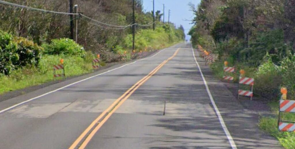
Jas. W. Glover, Ltd (Glover) paved a two-lane section of 1,300-foot on Highway 130 on the Big Island of Hawaii in June 2022. The scope of paving work included paving the Hot Mix Asphalt Base Course (HMABC) of variable thickness over the existing road to fill low areas and achieve the newly designed elevation. Glover decided to add a leveling course and a milling operation before the final lift was placed. The final lift was a 2-inch thick surface course (HDOT HMA mix IV). The project specification was based on the finished pavement meeting the fixed interval (or segmented) smoothness of MRI of 60 in/mi or under for every 0.1mile measured using a high-speed inertial profiling system.
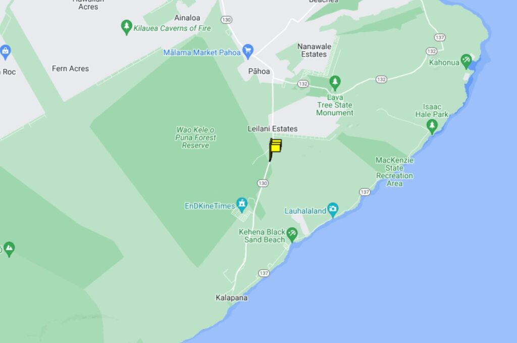
Project Location
Project Street View of Longer Wavelengths
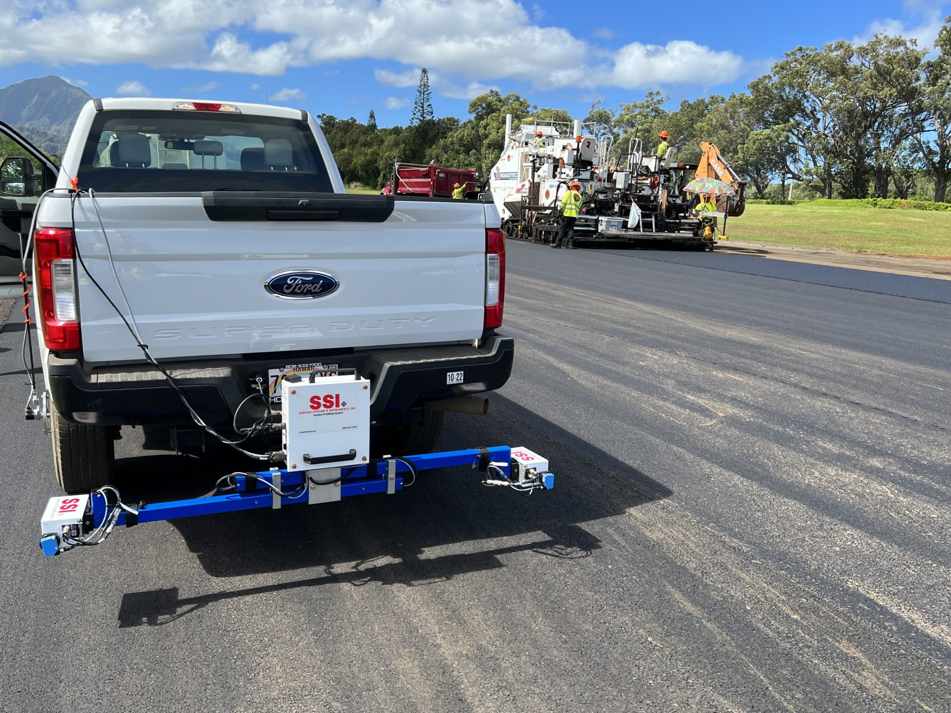
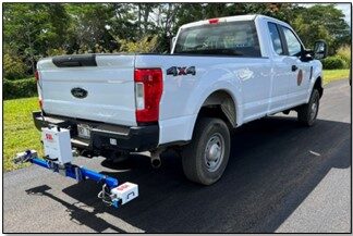
A portable bumper-mounted high-speed inertial profiler from Surface Systems and Instruments, Inc. was used to monitor the smoothness profile. Although it was not required to monitor smoothness after paving every lift, Glover’s quality control department collected smoothness data before the project started and after every phase of the project. The quality control team tracked the difference in smoothness between activities to provide the paving crew the baseline data before they advanced to the next activity. Jas. W. Glover Ltd.’s CS9300 Inertial Profiler is shown below.
Existing Data Analysis
The intention of the existing pavement analysis was to identify if the scope of work was adequate for the level of roughness and the cause of roughness. This step is all with respect to the final surface smoothness specification. Some of the knowledge is gained with experience, while other analysis methods were introduced to Glover by SSI technical staff. The identification of roughness from the profile data helps steer the paving crew in the right direction.
The smoothness analysis steps review:
- The existing MRI
- The short continuous roughness amplitudes (IRI ALR)
- MRI and IRI ALR final surface thresholds (i.e. improvement expected)
- Existing pavement distresses
- Wavelengths of the existing pavement surface
- Paving equipment to be used
- Mix design – typically the nominal aggregate size
- Planning (trucking, paving paths, cold joints, etc.)
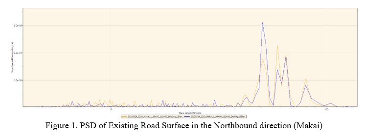
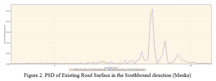
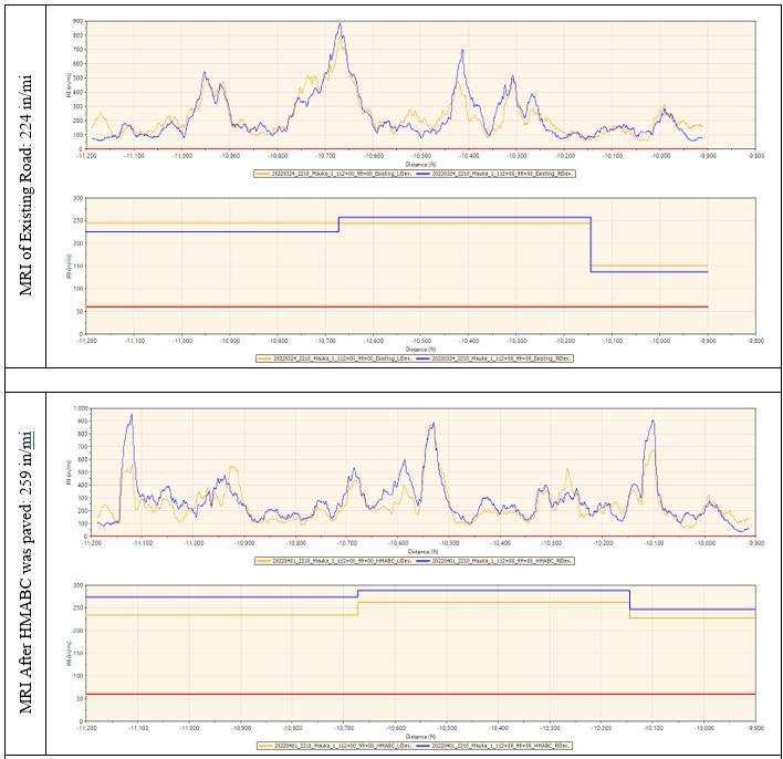
The existing road surface had an MRI of more than 220 in/mi on Northbound (Makai) and Southbound (Mauka) lanes. Glover’s QC team recognized that the lane roughness between each wheelpath was very consistent – the left and right wheelpaths had similar spikes in the same locations. This translated into the existing roughness being caused by undulations in the profile and not high frequency distresses like cracking and potholes. The Power Spectral Density (PSD) plots shown in Figures 1 and 2 confirm this for both Northbound and Southbound lanes. The orange and blue lines represent wavelength for the left and right wheelpaths, respectively.
The PSD plot is a common tool to identify wavelengths of features from electronic signals to pavement. Concrete pavement has many reoccurring wavelengths which show definitive spikes. The general rule of PSD plots is the larger the spike, the more impact that wavelength has on the profile. The PSD plots used for this analysis filter out the longer wavelengths outside of the IRI spectrum. This way, the largest spikes observed are the wavelengths with the largest influence on the IRI value.
PSD plots should be used to identify wavelength content and methods to remove them. IRI should not have any spikes near 7 or 50-feet. When deciding whether a project requires machine control, the focus should be on the left and right side of the PSD plot. When there are heavy concentrations of wavelengths on the right side of the plot, identifying longer wavelengths, then a 30-foot averaging ski will probably not remediate these undulations. If the project’s PSD plot only has high frequency chatter on the left side of the PSD plot, the averaging ski will probably be sufficient and machine control may not be required. All of these decisions depend on the variables of design, existing IRI of the roadway, construction restrictions, and the ability to collect accurate data for a machine control model.
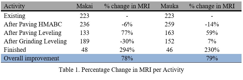
It is not uncommon for milled surfaces to have a higher IRI value than the existing surface. There is much more texture from voids and teeth marks on the milled surface. This is where the PSD plots are required to detect which wavelengths were corrected through the milling process for the contractor to project final smoothness. This can be seen within this project where the project smoothness progressed through the phases shown in Table 1 below. Even through a phase has a decrease in IRI smoothness because of adding short wavelength roughness, the final surface is actually improved because of the removal of longer wavelengths.
Intermediate Lift Analysis
After the existing analysis, the main goal of the intermediate lifts is to verify progress. The percent improvement of the roughness for your crew should be maintained along with improvement to the roughness that was expected to be reduced. It is recommended to verify the status after the last intermediate lift is placed.
Paving the Intermediate Lift
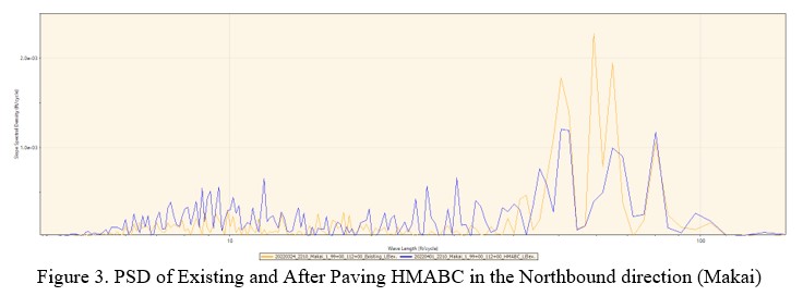
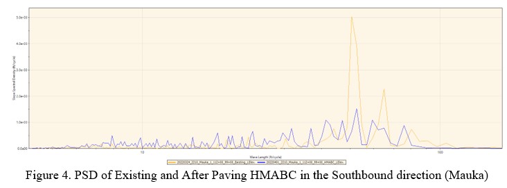
The asphalt base course (HMABC) – ranging from almost 0” thick to 12” thick – was paved over the existing surface to fill some large dips and connect the newly paved section to the existing road. The variable depth HMABC layer added slightly more roughness to the existing surface as it filled old dips and created new bumps. The PSD plots presented in Figures 3 and 4 illustrate this change for both lanes. For easy understanding of the plots, data from only the left wheelpath is plotted. The orange and blue lines represent the wavelength for existing and after paving HMABC, respectively. It is clear from the plots that some of the 50-foot wavelengths were removed after paving the HMABC (blue), while new high-frequency roughness was added (left side of plot).
Preparing for the Final Lift
Glover collected survey elevations to develop a final pavement elevation 3D model using Autocad Civil 3D. Based on the existing layer roughness, Glover engineers decided to pave a variable depth leveling course over the HMABC slightly higher than the finished elevation. This leveling course would be milled based on a 3D model to provide a surface to pave a consistent 2-inch thick final lift without an averaging ski.
A Trimble 3D machine control system employing total stations controlled the depth of the Roadtec milling machine. The width and length of this project was ideal for total station setup. A total station’s reach is only 350-500-feet, so multiple setups and mobilizations of the total station guns were required. The benchmarks and control points could be used for both sides of the two-lane road, which limited the setup work by the surveyor.
The Final Lift
Since the Glover QC team was monitoring the smoothness of each lift, they were more confident that the smoothness goal could be achieved. The added benefit of modeling and using machine control on the milling machine was that the final surface was more planar and level than an averaging ski surface. The paving crew had more consistent paving depths and less manual adjustments, contributing to the final smoothness success.
Project Phase ProVAL Data Plots
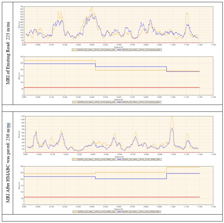
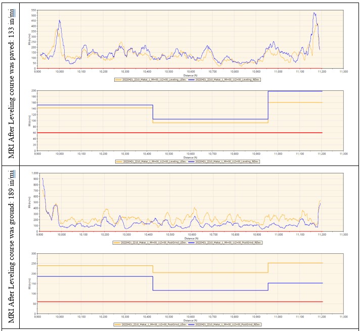
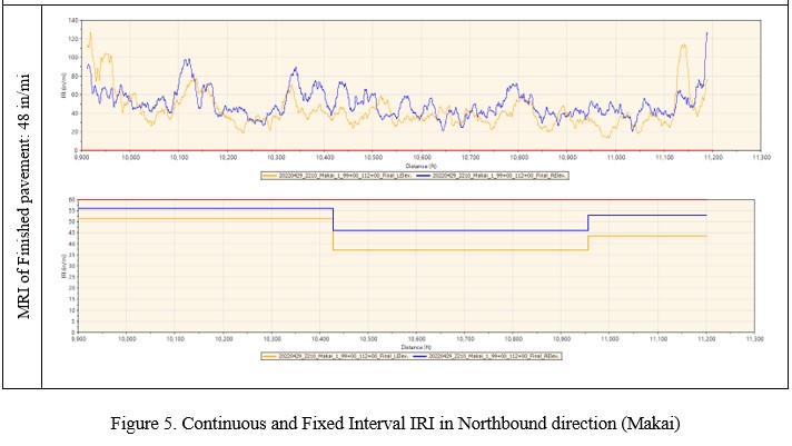
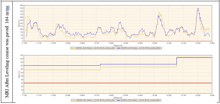
The plots included in Figures 5 and 6 show continuous IRI values per lane and fixed interval (or segmented) plot for every 0.1 mile for comparing the effect of each activity. The MRI of the road is also included to understand the improvement of each activity. As can be seen from the plots and MRI data, the existing pavement had MRI greater than 220 in/mi and the finished pavement had MRI less than 50 in/mi, which is an overall improvement of about 78%. The percentage change per activity is included in Table 1. It is clear from the table that although every activity has influenced the pavement smoothness. The biggest positive change can be seen with the final surface course paved over the ground leveling course. This demonstrates the importance of having a good underlying base to work on to achieve smoothness.
The list below shows when smoothness data was collected.
- Existing surface
- After HMABC was paved
- After Leveling course was paved
- After Leveling course was ground
- Finished pavement
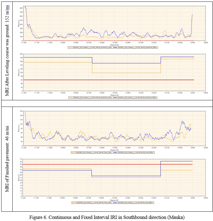
Figures 7 and 8 show the PSD charts for the four activities (existing, after paving HMABC, after paving leveling and after grinding leveling). The largest improvements are near 50-ft spike after paving the leveling course and after grinding the leveling course. The removal of the longer wavelengths allowed for the final surface to meet the project specifications
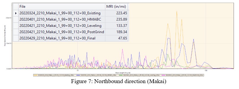
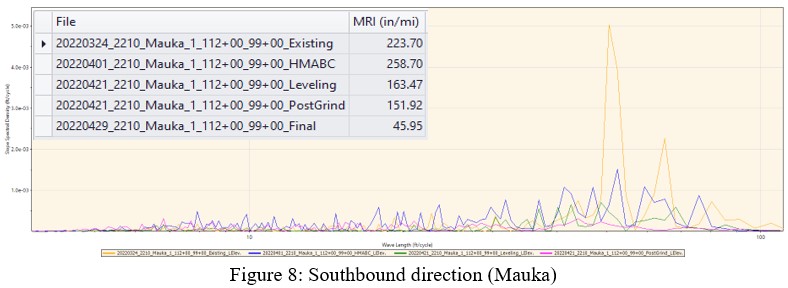
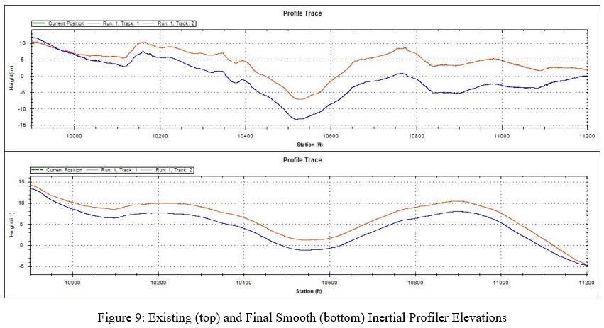
Figure 9 below displays the contrast between the existing (top) and the final (bottom) pavement elevation profiles. Each plot shows the left and right wheelpaths over the entire project limits. The inertial profiler is ideal for relative elevation measurement because of its high point density of 1-inch longitudinal sampling and sensors measuring vehicle elevation gains and pitch. The accelerometer and laser sensors of the inertial profiler can measure wavelengths over 5,000 feet long; well above the IRI wavelength limit of 250-feet (76-meters).
If success of the project can be shown in one graph, it is most clear within Figure 9. Through each phase of the project the rapid undulations of the existing profile have been replaced by steady, consistent vertical curves. The milling design was created to maintain the vertical curves and smooth out chatter within the elevation profile.
Final Improvement
Collecting smoothness information and sharing the data with the paving crew resulted in helping the paving crew adjust their paving operation based on their previous actions and procedures. Seeing the MRI numbers track in the expected direction also uplifted everyone’s morale. The MRI value of 48 in/mi and 46 in/mi in Makai and Mauka lanes, respectively, was under the project specification of 60 in/mi and amounts to an overall percentage improvement of over 78% for the project.
Without the leveling course, milling model, quality control, and proper planning for the stages of improvement, the specification’s MRI threshold of 60 in/mile may not have been met. The decision to collect MRI data after every activity proved to be valuable, as it provided important information to quality control department and the paving crew in making adjustments to the mix, paving and rolling operation. All these factors led to the project’s success.
Conclusion
Roads that are smooth and well-maintained offer a safer and more comfortable driving experience for motorists and contribute to the overall efficiency of the transportation network. As such, it is essential to prioritize smooth pavement construction and maintenance in road construction projects. With the smoothness specifications becoming increasingly more stringent, there are many tools a paving contractor can use to build a smooth pavement to meet the target specification. These tools range from a simple straightedge to verify behind a mill or paver, an inertial profiler, or pavement elevations from a survey or machine control model.
The success of this project can be attributed to several things, including placing the leveling course, using a model to mill the leveling course, good material and field quality control, using best paving practices, and proper planning for the stages of improvement. However, the most important takeaway from this project was the decision to collect smoothness data after every activity on the pavement. This proved to be critical, as the paving crew had quantifiable data to plan and adjust their procedures for the subsequent activity. Proper monitoring and control of all the above factors ensured the finished pavement met the specification’s MRI threshold of 60 in/mile or less.
Jas. W. Glover, Ltd. has been an SSI customer for over a decade. They have used the original California Profilograph and have been an early adopter during the Hawai’i DOT transition to inertial profilers. Mr. Rayapeddi Kumar has been involved with smoothness and partnered with SSI through these milestones. These are his experiences and lessons learned to achieve smoother pavements.